About the General Model Library
Coarsening Model
The Coarsening Property Model calculates the coarsening rate coefficient K (m^3/s) for secondary phases precipitating in a matrix phase during heat treatments, assuming spherical geometry of the phases. In the coarsening regime (where the driving force is capillarity), the change of mean particle radius evolves according to the equation for coarsening (or Ostwald ripening):
![]()
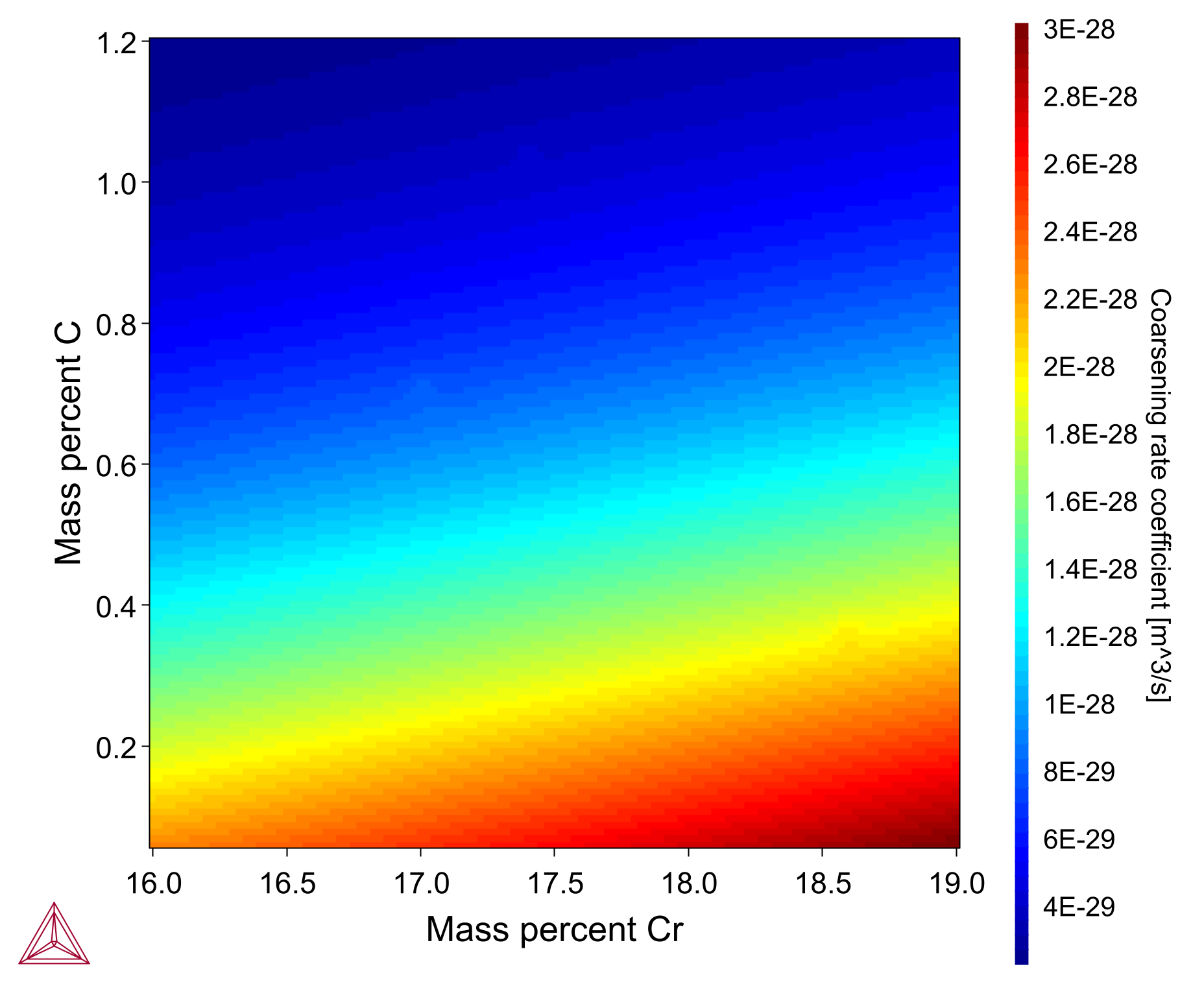
The heatmap plot shows the coarsening rate for an M23C6 carbide in an Fe-0.08C-1.4Ni-1Mn-17Cr nominal steel alloy with composition variation of Cr 16-19 wt% (X-axis) and C 0-1.2 wt% (Y-axis). The calculation is based on example PM_G_02 in the example files shipped with the software. A video is available demonstrating this model, which you can watch at the Property Model Calculator Video page.
Columnar to Equiaxed Transition (CET) Model
The Columnar to Equiaxed Transition (CET) Property Model calculates the fraction of equiaxed grains that correlates with a certain solidification condition, specifically thermal gradient (G) and solidification growth rate (v) (defined as the migration rate of the interface between liquid and primary solid), so that valuable information on the solidification microstructure can be obtained. The model formulation consists of two essential steps (1) to determine the dendrite tip radius and tip undercooling, and (2) to apply the calculated undercooling to the CET Model. Additionally, thermal gradient and solidification rates generated in the Additive Manufacturing Module can be overlaid over Columnar to Equiaxed Transition (CET) plots, allowing users to evaluate if the solidified microstructure corresponds to columnar or equiaxed, given the solidification conditions in the melt pool.
An example of the CET Model applied to additively manufactured IN718 is shown. In the top plot, CET curves show the typical thermal gradient and growth rate values for which columnar to equiaxed transition takes place, compared to experimental data. This example is available as example PM_G_17 in the example files shipped with the software.
The bottom plot shows the same CET simulation compared to solidification conditions at the melt pool calculated with the AM Module (blue points). When overlaid, it can be seen that nearly all the points (those below the purple line) exist in a fully columnar region. This calculation is available as example AM_10 in the example files shipped with the software.

Crack Susceptibility Coefficient Model
The Crack Susceptibility Coefficient (CSC) Property Model calculates the hot tearing tendency during solidification, also known as solidification cracking, hot cracking, supersolidus cracking, and shrinkage brittleness. The Model uses the Scheil Calculator to calculate the crack susceptibility coefficient, and the user can decide between three models, namely Clyne and Davies [1981Cly; 2006Yan], Kou [2015Kou], and Easton [2014Eas] models.
Hot tearing is one of the most common and serious defects encountered during the casting of, for example, aluminum alloys. Solidification shrinkage and thermal contraction occurs during solidification that leads to tensile deformation to cause cracking along grain boundaries that cannot be filled with remaining liquid.
The plot shows the CSC Model calculated for an Al-Si alloy using the Clyne and Davies model. The plot compares the predicted cracking susceptibility/composition curve for the Al-Si system with the experimental hot tearing tendencies. This calculation is available as example PM_G_07 in the example files shipped with the software. A video is available demonstrating this model, which you can watch at the Property Model Calculator Video page.

Driving Force Model
The Driving Force Property Model calculates the thermodynamic driving force for a phase divided by RT (R: universal gas constant and T: Temperature) to calculate the driving force per mole (J).
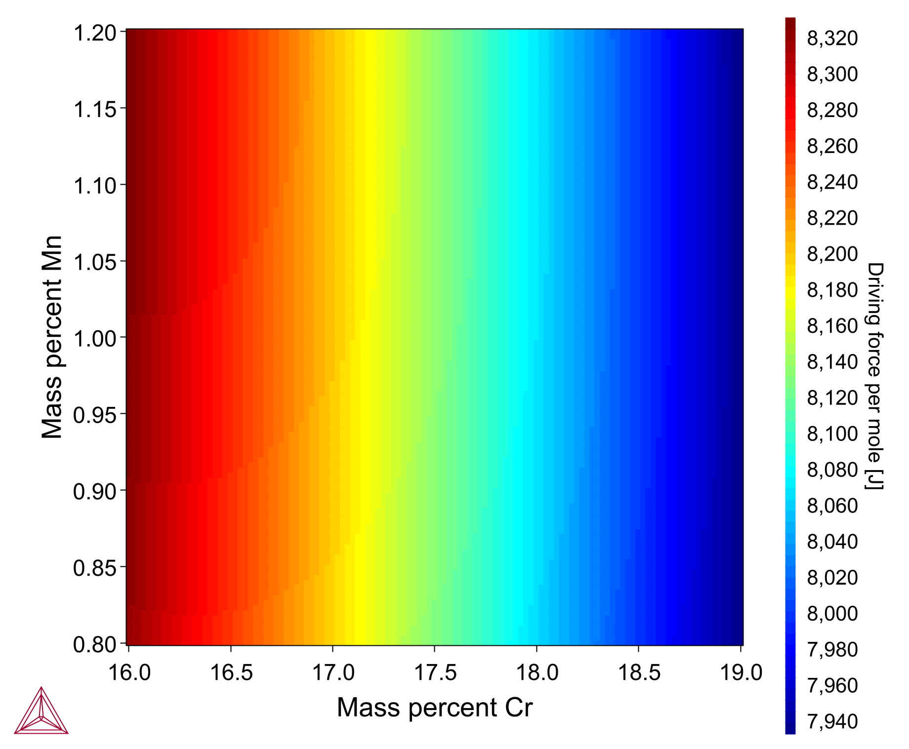
The plot shows how driving force of M23C6 precipitate varies as chromium (16-19 wt%) and manganese (0.8-1.2 wt%) composition varies in an Fe-17Cr-1.0Mn-1.4Ni-0.08C alloy. It is based on example PM_G_03, which is available in the example files shipped with the software.
A video is available demonstrating this model, which you can watch at the Property Model Calculator Video page.
Equilibrium Model
The Equilibrium Property Model calculates the equilibrium for the provided conditions. The calculation result from this model is the same as when you are using the Equilibrium Calculator with the Single Equilibrium calculation type, but this model is preferable when min/max or uncertainty calculations are required in case of compositional variations, which is true for most engineering materials.
An example for choosing annealing heat treatments for a medium carbon low alloyed AISI 4130 steel is shown. The alloy has the following composition, as per ASTM A29 standard:
| Fe | C | Mn | P | S | Si | Cr | Mo |
| Rem. | 0.28-0.33 | 0.40-0.60 | 0.035 | 0.040 | 0.15-0.35 | 0.80-0.10 | 0.15-0.25 |
The Equilibrium Model in this example is calculated for uncertainty in chemical compositions and annealing temperatures (820-900 ℃) to optimize for formation of austenite phase (FCC_A1). This is done to achieve microstructure suitable for machining. It is seen that best probabilistic results are achieved around 860 ℃, which agrees well with the industrially applied process. This model was calculated using the TCFE13 database in Thermo-Calc software.

Equilibrium with Freeze-in Temperature Model
The Equilibrium with Freeze-in Temperature Model calculates equilibrium at the freeze-in temperature and evaluates the properties at a different temperature. This model is particularly relevant for estimating thermophysical properties such as thermal or electrical conductivities. The assumption in this model is that diffusion and phase transformations are negligible when changing from the freeze-in-temperature and, therefore, that the phase amounts and compositions of phases are kept at all other temperatures.
The figure shows the thermal conductivity (W/m.K) as a function of temperature (℃) for an additively manufactured Cu-alloy (GRCop-42), which was developed by NASA for application in rocket engine combustion chamber liners. The values are compared against literature values [Chen2023] and show a good fit. This model was calculated using the TCCU6 database in Thermo-Calc. Note that this model uses thermophysical properties that are only available in some of the databases. If you are interested in this model, be sure to mention this to your sales agent.

Interfacial Energy Model
The Interfacial Energy Model is used to estimate the interfacial energy between a matrix phase and a precipitate phase using thermodynamic data from a CALPHAD database. The model is based on Becker’s bond energy approach [1938Beckers] and is also available in the Precipitation Module (TC-PRISMA).
In most situations, it is recommended to perform calibrations against some experimental data because the interfacial energy is dependent on many factors that are ignored in the estimation, for example entropy, incoherency, orientation, curvature, and so on.
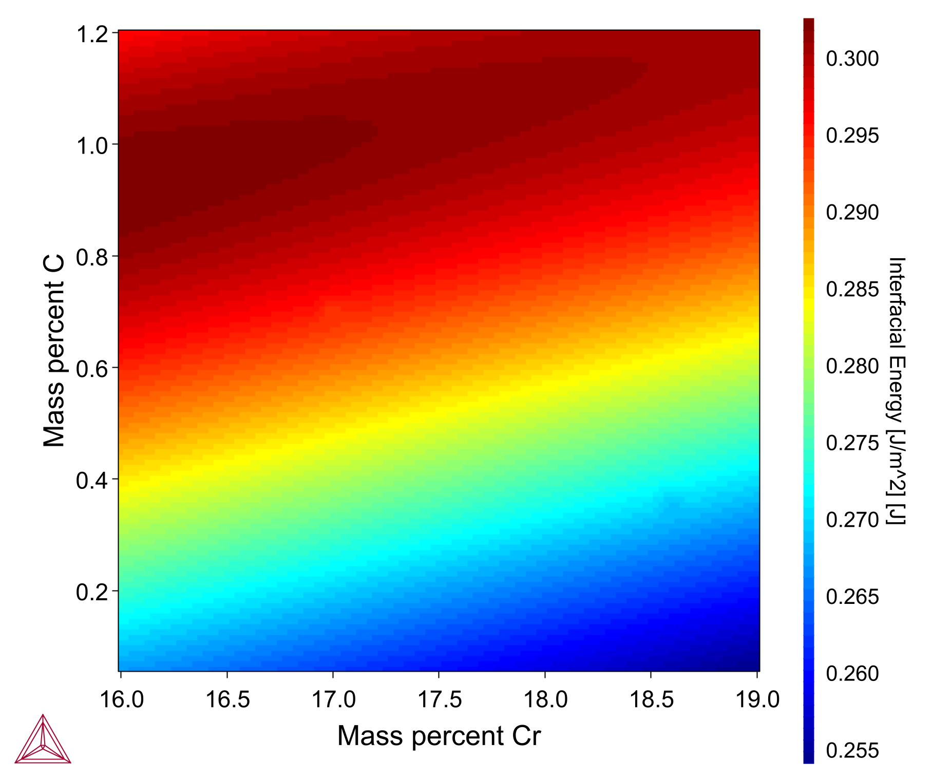
The heatmap plot shown here shows the interfacial energy for an M23C6 carbide in an Fe-0.08C-1.4Ni-1Mn-17Cr nominal steel alloy with composition variation of Cr 16-19 wt% (X-axis) and C 0-1.2 wt% (Y-axis). It is based on example PM_G_02 in the example files shipped with the software.
A video is available demonstrating this model, which you can watch at the Property Model Calculator Video page.
Liquidus and Solidus Temperature Model
The Liquidus and Solidus Temperature Model is a Property Model that calculates the equilibrium solidification range for a given alloy. For example, you can easily use uncertainty calculations, varying one or more conditions such as composition range, and see how that affects the liquidus and solidus temperatures.
The plot shows a comparison of experimental liquidus and solidus data using a cross plot with a batch calculation. A root mean square (RMS) setting shows the error distribution of the data points. The alloy studied is Fe-C-Cr-Mn-Ni with C: 0.22-0.72 wt%, Cr: 1.47-4.21 wt%, Mn: 0.47-1.08 wt% and Ni: 0.82-2-6 wt%. The plot is based on example PM_G_12, which is included in the software.
A video is available demonstrating this model, which you can watch at the Property Model Calculator Video page.
You can also see an example of the model in use on the Powder Metallurgy page.

Phase Transition Model
The Phase Transition Property Model calculates the point when a new phase may form by varying set conditions. The model is useful to determine melting temperature, boiling temperature, or solubility limits. It returns the phase transformation temperature, or composition, depending on the varied condition.
The plot is a histogram showing how the transition temperature (℃) of sigma phase varies when you vary the composition for an Fe-1.4Ni-0.08C-1.0Mn-17Cr alloy. The plot is based on example PM_G_01 of the examples included in the software.
A video is available demonstrating this model, which you can watch at the Property Model Calculator Video page.

Scheil Model
The Scheil Property Model calculates solidification under the Scheil assumption. This Property Model is essentially the same as the Scheil Calculator included in the software, but implementing Scheil as a Property Model allows users to benefit from the additional calculation types available in the Property Model Calculator, including multi-axis Grid, Min/Max, Uncertainty, and Batch.
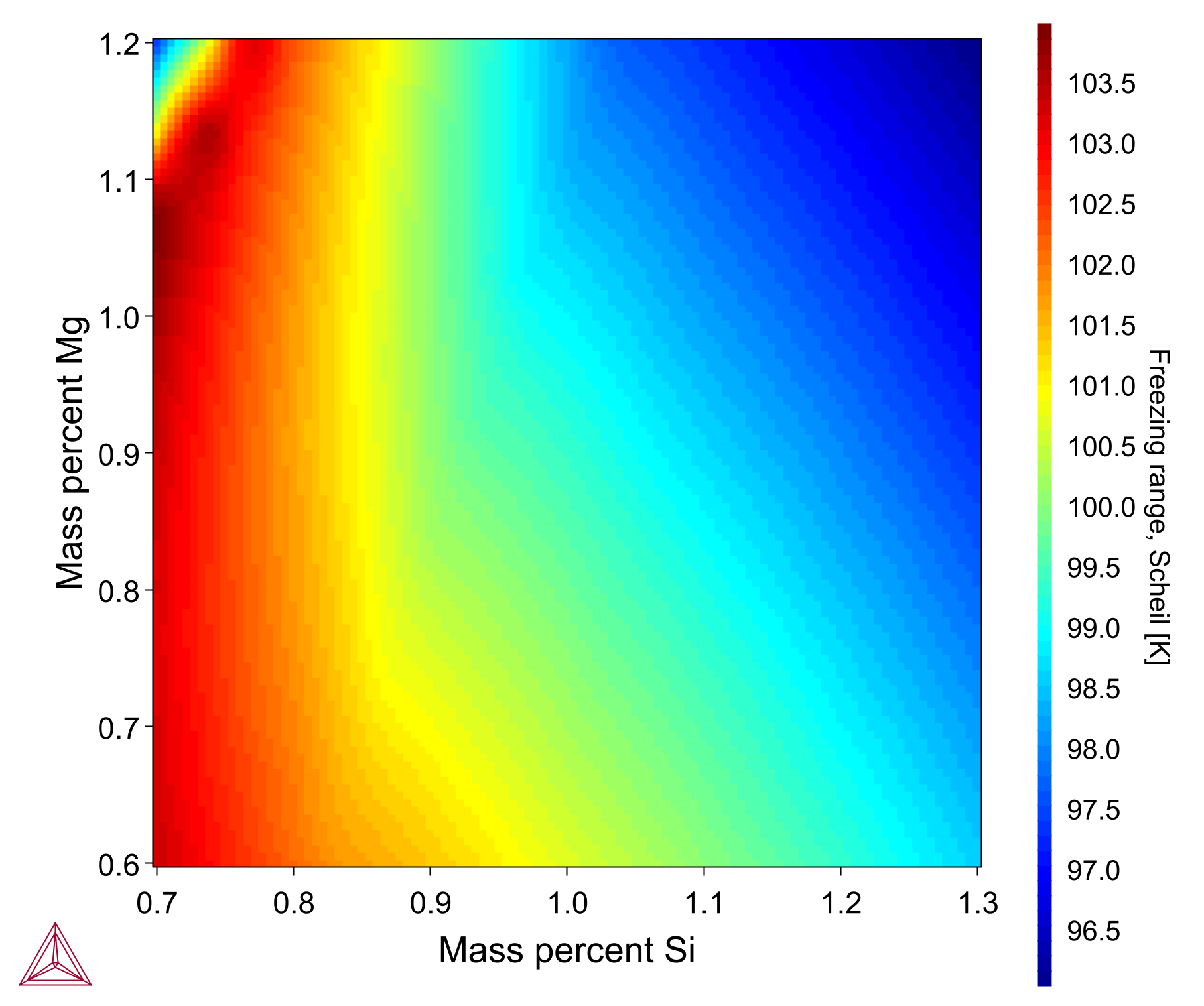
The heatmap plot considers an Al-1Si-1Mn-0.7Mg-0.6Fe-0.1Cu alloy wherein the freezing range is plotted with respect to changing chemical composition of Si (0.7-1.3 wt%) and Mg (0.6-1.2 wt%). The calculation is made with the TCAL9 database and Thermo-Calc software.
Spinodal Model
The Spinodal Property Model calculates the spinodal line, which is defined by the condition where the second derivative of Gibbs free energy is zero (d2G/dx2 = 0). The locus of these points is known as the spinodal curve. With this Model, up to two spinodal solutions can be found. When searching for the spinodal, users can vary the temperature or a composition in mass percent, mole percent, mass fraction, or mole fraction.
The plot shown here is a binary Fe-Cr spinodal curve for BCC that goes through the one-phase region for Sigma. This example can be found as example PM_G_08 in example files provided with the software.

T-Zero Temperature Model
The T-Zero Temperature Property Model calculates the so-called T0 line, which is defined as the temperature where two phases of identical chemical composition have the same molar Gibbs free energy. This temperature is an important quantity in the field of diffusionless phase transformations, such as martensitic transformation, since it is the upper limit where diffusionless phase transformations can occur.
The plot shows the Fe-Ni binary system wherein the T0 line for the FCC_A1 and BCC_A2 phases is located in the middle of the two-phase region. No solution for the T0 temperature exists above about 30 mass% Ni. This example can be found as example PM_G_09 in example files provided with the software.

Yield Strength Model
The Yield Strength Property Model is a general model to estimate the expected yield strength of a material. It considers four contributions to the overall yield strength of the material: intrinsic strength for the pure elements, grain boundary strength (Hall-Petch effect), solid solution strengthening, and precipitation strengthening. The temperature (intrinsic strength) is used to evaluate the equilibrium state of the system, and the resulting compositions and phase fractions are subsequently used in the evaluation of mechanical properties.
The top plot shows a solid solution strengthening example wherein yield strength vs Ta-content for the binary high entropy Mo-Ta alloy is compared to experimental data at 300K and 411 K [2017Wal]. The plot is calculated using the TCHEA7 database in Thermo-Calc and is based on example PM_G_06.
The bottom plot shows a precipitation strengthening example wherein yield strength v/s mean radius for a binary Al-0.3Sc alloy is shown and compared to experimental values [2002Seidman]. The plot is based on example PM_G_04 of the examples shipped with the software.


Run the Examples Yourself
Several examples are included in the software to help you get started using the General Property Models. Most of the examples use DEMO databases, so they can be run by all users, regardless of which databases you purchase.
If you do not already have a license for Thermo-Calc, many examples can be run in the Free Educational Package.
Some of the examples also have accompanying videos that walk you step-by-step through setting up the calculation in the Property Model Calculator and include interpretation of the results.
