
Getting Started with Thermo-Calc

Welcome to the Getting Started Guide for Thermo-Calc

This guide is for those who are new to Thermo-Calc and want a quick guide to get started with your calculations within Graphical Mode. You will learn how to navigate within the program and how to set up a simple calculation with our different Templates offered in the Graphical Mode. 

Use the side menu to the right to navigate through the different parts of the guide, or read the entire guide by just scrolling down on this page. You can also watch the Getting Started Video available at the top of this page. 

We hope you will find this guide helpful! 

Before you begin, make sure that you have the Thermo-Calc software installed on your computer, either the full package or the free Educational Package. If you need help with the installation, read our installation guide or watch our installation videos.

Getting Started Guide for Thermo-Calc Video

The Thermo-Calc Getting Started Guide is also available as a video, which contains the same content as this web page.

Overview of the Calculators and Add-On Modules

When you first open the Thermo-Calc software, a window with all the different templates will show up in the center of your screen. It is called the Configuration Window.

01_homepage

At the top of the Configuration window, you will find resources to help you learn about the program, such as a Getting Started Guide and the Online Help.

Below that, you will find templates showing the different calculators available in Thermo-Calc as well as the Add-On Modules, which require additional licenses. The license requirements are described directly below. 

Templates Included in Thermo-Calc Graphical Mode

Calculators in Thermo-Calc:

  • Single Point
  • One Axis
  • Material to Material
  • Phase Diagram
  • Binary
  • Ternary
  • Scheil Solidification
  • Property Models

The calculators can be run by anyone with a Thermo-Calc license, including the Educational Package.

Add-On Modules:

  • Diffusion Module (DICTRA)*
  • Precipitation Module (TC-PRISMA)*
  • Process Metallurgy Module*
  • Steel Model Library (Steel TTT, Steel CCT)**
  • Nickel Model Library**
  • Additive Manufacturing***

*Can run simulations with up to three elements using the included DEMO version of the Module. Larger simulations require a license for each Module.

**Additional license required to run any calculation.

***Requires additional license and at least one thermodynamic and properties database that includes the necessary properties data.

Educational Package

The Educational Package is a limited version of Thermo-Calc that is intended only for educational purposes in an academic environment. The Add-On Modules included are:

  • Diffusion Module (DICTRA)
  • Precipitation Module (TC-PRISMA)
  • Process Metallurgy Module 

The Educational Package is limited in the sense that calculations can only handle three components or fewer.

The Steel Model Library, Nickel Model Library, and Additive Manufacturing Module are not included in the Educational Package and can not be used to run calculations without a license.

How to Set Up a Thermo-Calc Calculation

Open the Thermo-Calc software and make sure you are in Graphical Mode. If you happen to be within the Console Mode, you can click this button screenshot of the switch to graphical mode button to switch to Graphical Mode.

In this guide, we will show you the basics of how to set up a One Axis Equilibrium Calculation and view the result both as a plot and a table.

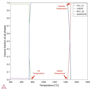
A one axis calculation is very useful to get information about how the phase structure of the material varies with temperature. For example, it can be used to find the suitable temperature range for forging applications. From this calculation, we can also read the liquidus, solidus, and any transformation temperatures. In the example below, we will demonstrate how to use this calculation to find the A3 temperature, an important transformation temperature in steels, for a Fe-C alloy.

Choose Template

02_one-axis

The different templates offered in Thermo-Calc are shown in the Configuration window in the center of the screen.

Select the template you want to use by double-clicking on it. For this example, click the One Axis template.

01_project-tree_2024a

A series of icons, known as Activity Nodes, are shown in the Project window on the left side of the software, as seen in the figure here.

When you work in Thermo-Calc, you work in projects. Each project consists of a set of linked Activity Nodes. In order to set up a calculation, you must configure each node, which we will do in the following steps.

The easiest way to set up a calculation is to use the templates, but you can also set up the calculation by right-clicking on any of the nodes in the Project window and adding subsequent activity nodes one by one.

Some of the nodes also have yellow icons on them. These symbols tell you the status of that node, for example, the yellow exclamation point indicates that the node needs to be configured, a pink clock appears while the calculation is running, and a green checkmark appears when the calculation is done. 

Select Database and Material Composition

To run a calculation, you need to select an appropriate database and define your material. This is done in the System Definer.

Step 1

Open the System Definer by clicking on the System Definer-node

Step 2

To select the database, click on the drop-down list below Databases in the Configuration window.

For this calculation:

  • Select the FEDEMO database. This is a free database included in all installations. You could also select any version of the TCFE databases if you have that included in your license.
Step 3

Select the elements that you want to include in your calculation. Make sure to select the dependent variable first.

For this calculation:

  • Select iron (Fe) first since that is our dependent variable.
  • Select carbon (C) as the second element.
Step 4

Change the composition for your material by changing the numbers in the text box to the right of the Configuration window.

For this calculation:

  • Change the carbon content to 0.5 mass percent. The iron content will be balanced based on the carbon content that you enter since iron was selected as the dependent variable.

Set Up the Conditions

The next step is to set up the conditions for your calculation. This is done in the Equilibrium Calculator, so click on that node. 

In the Equilibrium Calculator, you can change the conditions for your calculation, such as temperature, pressure, system size, composition. You can also change which calculation type you want to use and the axis definitions.

For this calculation:

  • Change the temperature unit to Celsius.
  • Make sure that the One axis calculation type is selected.
  • Change the temperature range to 400-1800 oC under Axis Definitions.
  • Leave the rest as default. You can use the screenshot to make sure your defaults match mine.

Screenshot showing how to configure the Equilibrium Calculator in Thermo-Calc.

The values in Condition Definitions are used as a starting point for the calculation. It is important that these values are within the range set in Axis Definitions, in this case the temperature.

Run the Calculation and View the Results

The results can either be viewed as a plot or a table. When using the One Axis template, the default is to use a Plot Renderer. 

View the Results in a Plot

In the Plot Renderer node you can change the axis variables by clicking on the Axis variable drop-down lists.

For this calculation:

  • Select Temperature as the X-axis variable and Celsius as the unit.
  • Select Volume fraction of phase as the Y-axis variable and select All phases.

By unticking the Automatic scaling box, you can adjust the scale for each axis. This is not always necessary but is useful if you want another scaling than the one automatically generated. We will leave it checked for this calculation.

Screenshot showing how to manually change the axis scaling in Thermo-Calc.

When everything is set-up, click the Perform button in Thermo-Calc button on the bottom of the program to run the calculation. 

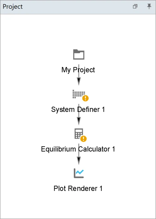
When the calculation is running, the Event Log will start populating and clocks will appear on each activity node in the Project window. The calculations may take several minutes to run depending on the type of calculation.

Once the calculation is done, the results will appear in the Visualizations window.

Results shown as a plot in the visualizations window.

Interpretation of the Result

According to this diagram, the steel will solidify as FCC phase (blue line) and we will have a region with 100% FCC before BCC starts to form. At 1498°C we have the liquidus temperature, which is found where the red line reaches 1 mole. The solidus temperature is found where the amount of liquid is zero, which is around 1436°C. The BCC phase (green line) starts to form at around 770°C and this is where we find the A3 temperature.

Interpretation of results from step calculation in Thermo-Calc.

View the Results in a Table

If you want the result shown in a table, you can easily add a Table Renderer by right-clicking on the Equilibrium Calculator node > Create New Successor > Table Renderer, and the Table Renderer node will appear in the Project window.

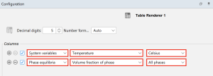
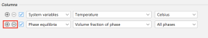
In the Table Renderer node you can select the different properties you want to show in the columns of the table by clicking on the drop-down list.

For this calculation:

  • Select Temperature in Celsius for the first column.
  • Select Volume fraction of phase and All phases for the second column.

Screenshot showing how to change the axis variables in Thermo-Calc.

You can also add more columns by clicking on the plus sign and remove columns by clicking on the minus sign.

Screenshot showing where to add more columns to the table.

When everything is set-up, click the Perform button in Thermo-Calc button on the bottom of the program to run the calculation. 

Once the calculation is done, the results will appear in the Visualizations window.

Results in table format in the visualizations window.

Table View Option

As of the 2022a release, you can choose to view your plotted result in a table directly in the Plot Renderer. This provides a quick and easy way to view a table without creating another node. 

To do this, return to the Plot Renderer node and select the Table View option in the top menu of the Configuration window then click Perform at the bottom, center of the program. Your plot will be replaced with a table.


Save the Results and the Project

After your calculation is done, you can save the results locally on your computer or cloud services.

Save the Plot

Step 1

Depending on which window you are in:

  • In the Visualizations window, right-click the diagram and select Save As…
  • In the Configuration window you can also click the Save Diagram buttons to open the Save window.
Step 2

In the Save window:

  1. Navigate to where you want to save the diagram.
  2. Enter a file name.
  3. From the Files of Type list choose png (the default), jpg, ps, pdf, gif, svg, or emf.
  4. You can set the resolution of the image by unchecking the Use default resolution box and setting a different resolution.
  5. When you are ready, click Save.

Save the Table

Step 1

Depending on which window you are in:

  • In the Visualizations window, right-click the diagram and select Save As…
  • In the Configuration window you can also click the Save table button to open the Save window.
Step 2

In the Save window:

  1. Navigate to where you want to save the diagram.
  2. Enter a file name.
  3. From the Files of Type list choose Text [*.txt](the default), Hyper Text Markup [*.html], or Excel [*.xls].
  4. When you are ready, click Save.

Save the Project

In Graphical Mode you work with one file type, a project file, which has a *.tcu file extension. This is applicable to Thermo‑Calc and all of the Add-on Modules.

Step 1

Navigate to the top menu and select File > Save Project or Save Project As…

Step 2

In the Save Project window:

  1. Navigate to where you want to save the table.
  2. Enter a file name.
  3. When you are ready, click Save.

If you want the results to show up the next time you open the file, without having to run the calculation again, you can select the Include calculated results in the project file option at the bottom of the Save Project window. This will save you time when you open the file, but will result in a larger file.

Screenshot showing how to include the results in your project file.

Perform Parallel Calculations

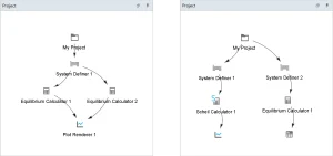
If you want to combine calculations, you can add additional activity nodes to your project to link information. For instance, you can add two calculators to one plot to compare the results. The example video T_05 – Stable and Metastable Phase Diagrams, shows how to plot a metastable and a stable phase diagram in two separate plots and how to combine them into one single plot.

These images show two examples on how you can combine different activity nodes to perform several calculations in one single project.

Two screenshots showing how to connect different nodes to perform parallel calculaitons.

How to Run the Example Calculations

Your Thermo-Calc installation includes example files with different types of calculations, which you can use to learn how to use the software. 

Example calculations for both Graphical Mode and Console Mode are included in your installation. 

To run the example calculations within the Graphical Mode, open your software and follow these steps:

Step 1

On the homescreen of the software, click the Example Files icon.

or

Navigate to the top menu and click Help > Example Files…

Step 2

A pop-up window will appear, showing folders with calculations for the different modules. Navigate through the folders, select the calculation you want to run, and click Open.

Step 3

When the example file opens, the different activity nodes will appear in the Project window. To run the calculation, right-click on the top node and click Perform Now.

Once the calculation is done, the result is displayed in the Results window

Many of the examples have a corresponding video, which can be found on our webpage and Youtube channel.


Thermo-Calc Examples  |  Diffusion Module (DICTRA) Examples  |  Precipitation Module (TC-PRISMA) Examples  |  Property Model Calculator Examples  |  Process Metallurgy Module Examples

Useful Tips & Tricks

This section includes tips and tricks that can be useful for you as a Thermo-Calc user.

Rename the Nodes 

When working with projects in Thermo-Calc, it can be helpful to rename the different activity nodes. This is especially useful when working with larger projects where you do several calculations in parallel. 

To rename an activity node you simply right-click on the node in the Project window and select Rename. Write the name of the node in the textbox and click OK

Save the project as usual. 

Once you reopen your project, the name of your nodes will be the same as when you saved the project.

Save the Project With Notes

For every activity node, you can write down notes that are saved with your project. This can be information that you want to remember the next time you open the project or, if you share the project with others, something that someone else should read when they open the project.

Go to the activity node where you want to add a note. Click on the page button at the bottom of the Configuration window. Save your project as usual and the note will be saved with your project file.

Customize the Plot

Before saving your plot, you can customize the appearance of the plot. 

  1. Right-click on the plot 
  2. Click on Properties

In the Plot Properties window, you can edit fonts and font size for the labels, legends, and titles. You can also change the line thickness, color, and more.

Play around with the settings and see what settings are best for your purpose. 

As of  the 2022b release, you can use themes to save your plot settings. This is especially useful if you need consistent looking plots, for example, for a presentation, publication, or collaboration. The theme settings are located at the top of the properties window. You can either use the predefined plot themes or define your own themes.

You can read more about the themes by searching for Plot Themes in the online help. The online help is accessed from within Thermo-Calc in the Help menu > Online Help

Add Labels to the Plot

You can also add labels to your plot.

  1. Right-click on the plot
  2. Click Add Label… 
  3. Write the name of the label in the text box 
  4. When you are ready, click OK
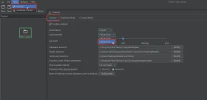
Dark Mode

Dark mode is available in Graphical Mode as of Thermo-Calc 2023a. To switch to dark mode, go to Tools in the top menu of the software and click Options. Next to Look and feel in the Options window, select FlatLaf Dark in the drop-down list and click OK.

A screenshot showing where to switch to dark mode in the graphical user interface of Thermo-Calc.

Where to Find Help and Resources

Online Help

In the online help, you can browse the menus and search for keywords and phrases to find the information you are looking for. It contains the same documentation that is also installed in folders with your software. The online help system opens in your internet browser, but the files are stored locally on your computer, so you do not need an internet connection to use it.

The online help is accessed from within Thermo-Calc in the Help menu > Online Help.

Example Calculations

All Thermo-Calc installations include example files for both Graphical Mode and Console Mode. The Graphical Mode examples are available for Thermo‑Calc and the Add-on Diffusion Module (DICTRA), Precipitation Module (TC-PRISMA), Process Metallurgy Module, and Additive Manufacturing Module. There are also examples for the Property Models, including the Steel Model Library and more. The Console Mode examples are available for Thermo‑Calc and the Diffusion Module (DICTRA). 

The example files are found by navigating to the Help menu > Example Files…

If you are in Console Mode, the console mode examples will open, and if you are in Graphical Mode, the graphical mode examples will open.

Application Examples 

Our Application Examples show how Thermo-Calc can be used to improve products, optimize materials processing conditions, and give you a deeper understanding of materials. Each example includes an in-depth PDF and calculation file, which are included in your software installation and can be run if you have a license for the relevant products. 

You can find the Application Example PDFs on our webpage

Video Tutorials

We provide videos explaining how to make different thermodynamic calculations, diffusion simulations, and precipitation simulations using Thermo-Calc software. Our videos will also teach you how to install Thermo-Calc and will keep you up-to-date on the latest releases and additions to the software and the newest thermodynamic, properties, and kinetic databases.

Visit our Video Tutorial Library

Learning Hub

The Learning Hub includes courses for Thermo-Calc, the Diffusion Module (DICTRA), the Precipitation Modules (TC-PRISMA), and the TC-Python SDK. In addition to introductory lectures, instructors walk through and discuss real-world examples that correlate calculations with microstructures and other metallurgical concepts, spanning a wide range of material types. Our team is working on adding content for additional modules, so make sure to check back regularly.

Visit the Thermo-Calc Learning Hub

Training Courses 

Thermo-Calc Software offers Live Online Training several times throughout the year for Thermo-Calc, the Diffusion Module (DICTRA), and the Precipitation Module (TC-PRISMA). We can also provide Customized Training upon request. We also support Third Party Training and Workshops, which are listed on our website.

Learn more about our Training Courses

Let Us Help You

Is Thermo-Calc Right for You?

Talk to one of our experts to learn whether our tools fit your needs.