Welcome to the Getting Started Guide for the Diffusion Module (DICTRA)
About this Guide and the Example Calculation
This guide will cover the general procedure of how to set up a basic DICTRA calculation by guiding you through the set-up of a calculation example of a Fe-Cr-Ni diffusion couple with different nickel contents.
The diffusion couple consists of two foils of different materials in the same phase, Austenite (FCC), but with different compositions. The two foils are joined together and kept at an elevated temperature of 1200 K.
The simulation is set up as a single region calculation with a step in the composition profile where the different materials meet. The material on the left side is Fe-18Cr-8Ni and the material on the right side is Fe-18Cr-26Ni. The thickness of each of the two foils is 50 micrometers. The image shows an illustration of the two foils where the Ni content is indicated with a blue dotted line.
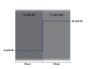
A schematic illustration of the diffusion couple.
Add the Necessary Nodes and Define the Initial System
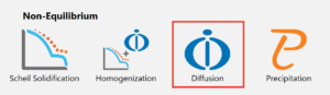
On the home screen of Thermo-Calc, click the Diffusion template to add the necessary activity nodes.
Select Databases and Elements
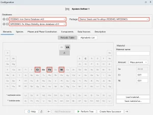
In the System Definer node, select the suitable databases and elements for your simulation. Since you are going to perform a diffusion simulation, you need both a thermodynamic and mobility database. Under the Databases dropdown menu, click the plus sign to add a second database or choose a database package.
For this example:
Select Phases
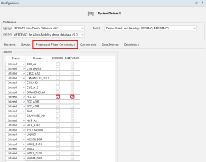
Diffusion simulations can sometimes be quite demanding and take a long time to run. It is therefore recommended to deselect the phases that are not necessary for the specific calculation. In the System Definer, click on the Phases and Phase Constitution tab and deselect all phases that are not necessary for your calculation.
In this example, we will calculate at a temperature of 1200 K, and the material will be fully austenitic (only FCC phase) at that temperature. Therefore:
Note: To know which phases are present in your material at a specific temperature, you need to perform an equilibrium calculation in Thermo-Calc, for example, a phase diagram. On the home page of the software, there is a Phase Diagram template that is useful for this kind of calculation. You can also watch our video demonstrating how to calculate a binary phase diagram.
Select Units
In the Diffusion Calculator, you can set which length and composition units you want to use for your calculation. The default units are mass percent (wt%) and meter (m).
For this example:
Select Geometry
The Diffusion Module handles diffusion problems where composition varies along one spatial coordinate. You can choose planar, cylindrical, or spherical geometry.
For this example:
More About the Geometries
Planar
Cylindrical
Spherical
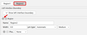
Define a Region
For diffusion simulations, at least one region should be defined containing at least one phase. For some calculations, you might want to create several regions, for example moving phase boundary simulations. Naming the regions is optional, but can be useful when having more than one region. To add a new region, click the plus sign next to Region. In this example, we will not add a second region.
For each region, select which phase is present in the region and enter the composition profile. You should also select a grid type for each region. There are three grid types available: linear, geometric, and double-geometric. You can also select to have the program set the grid points automatically.
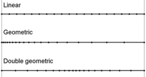
For this example:
Define the Composition Profile of the Region
In the Phase drop-down list, select FCC_A1. The composition profile settings now appear below the Region box, and a visualization of the composition profile is shown in the Visualizations window. Select the dependent component, usually the majority element, and edit the composition profile for the other components in your system. You can choose either Linear or Step composition profiles, or describe the composition profile with a Function.
In this example, we will simulate how the Ni content varies between the two metal sheets with different Ni concentrations.
This will create a composition profile that simulates two materials with different nickel compositions, i.e. one with 8 wt% nickel and one with 26 wt% nickel. The composition profile is shown in the Visualizations window.
Note that the step in the center is not a phase interface, our setup represents a single phase FCC structure with a concentration jump.
For this calculation:
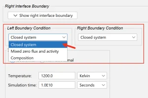
For more details about boundary conditions, read the Diffusion Tutorial or search for boundary conditions in our Online Help, which is accessible from within the software.
For this example:
Run the Calculation and Visualize the Result
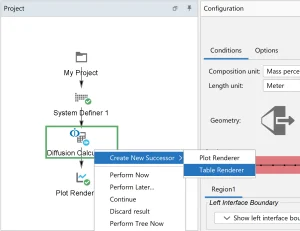
The last step before running the calculation is to choose how you want to visualize the result, either with a plot or a table. When using the Diffusion template, the default is that a Plot Renderer is added to the project tree. If you want your results in a table, you can simply add a Table Renderer by right-clicking on the Diffusion Calculator, then click Create New Successor > Table Renderer.
Learn more about how to visualize the results in the Thermo-Calc Getting Started Guide.
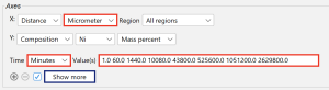
The major difference between the Plot and Table Renderers in DICTRA compared to Thermo-Calc is that you need to set the time(s) you want to show, unless you use time as the x-axis unit. In the box right below the axis setting, write the time you want to visualize in the text box. This applies for both the Plot Renderer and the Table Renderer. It is important that this time is shorter or equal to the simulation time you set in the Diffusion Calculator, otherwise, it can not be shown since DICTRA does not have any calculated values at those times. If you want to show the results at different times, you can separate the times with a space. You can choose to set the time in seconds, minutes, hours, or days.
For this example:
Click ![]() at the bottom of the Plot Renderer window and see that the event log starts populating. When the calculation is finished, the result will show in the Visualizations window.
at the bottom of the Plot Renderer window and see that the event log starts populating. When the calculation is finished, the result will show in the Visualizations window.
Interpretation of the Result
In the plot, it is shown that when the diffusion couple is held at an elevated temperature (1200K) for a more extended period of time, the nickel will diffuse from the nickel-rich to the nickel-poor material and we get a composition gradient on both sides. It is also shown that it takes around 5 years for the diffusion couple to get a homogeneous nickel content, that is the nickel content in both materials is the same.