Thermo-Calc 2025b Available Now
Webinar on Thermo-Calc 2025b Release
Discover what’s new in Thermo-Calc 2025b in our on-demand release webinar. Explore powerful new features, updated databases, and enhancements designed to improve your workflow. Get firsthand insights from three of our developers as they walk you through the key innovations in this latest release.
Databases and Thermophysical Properties
New Databases
TCMG8: Mg-based Alloys Database
The database has been enhanced to perform rare earth (RE) calculations for Mg-RE-Sn systems (RE=Ce, La, Nd, Pr).
Updated Databases
MOBSLD2.1: Solder Alloy Solutions Mobility Database
MOBSLD2.1 is available for free to everyone who has MOBSLD2 and a current Maintenance & Support Subscription.
Restructured Quantities List for Improved User Experience
Finding the right plot and table variables has become easier in this release. With over 50 options available, the quantities have been reorganized into helpful categories for quicker navigation. Additionally, the software now filters the list to display only the quantities available in the databases being used.
The full variables list is still available for users who prefer to see all the variables in one alphabetized list.
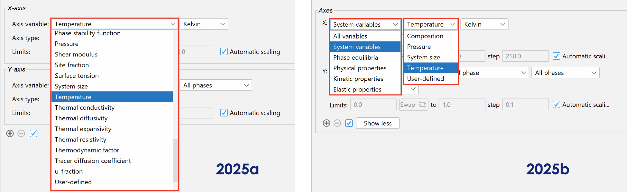
Left: Results quantities list in Thermo-Calc 2025a, showing over 50 options in a single, ungrouped list. Right: Results quantities in 2025b, now organized by category for easier navigation.
Database Properties Displayed in System Definer
As we’ve continued adding properties to our databases, it’s become increasingly difficult to keep track of which databases include which properties. With this release, that changes: now, when you select a database in the System Definer, its available properties are listed in the same window, making it easier than ever to find the information you need.
Note that the software simulates many more properties than those listed. The list only includes database-specific properties, which are:
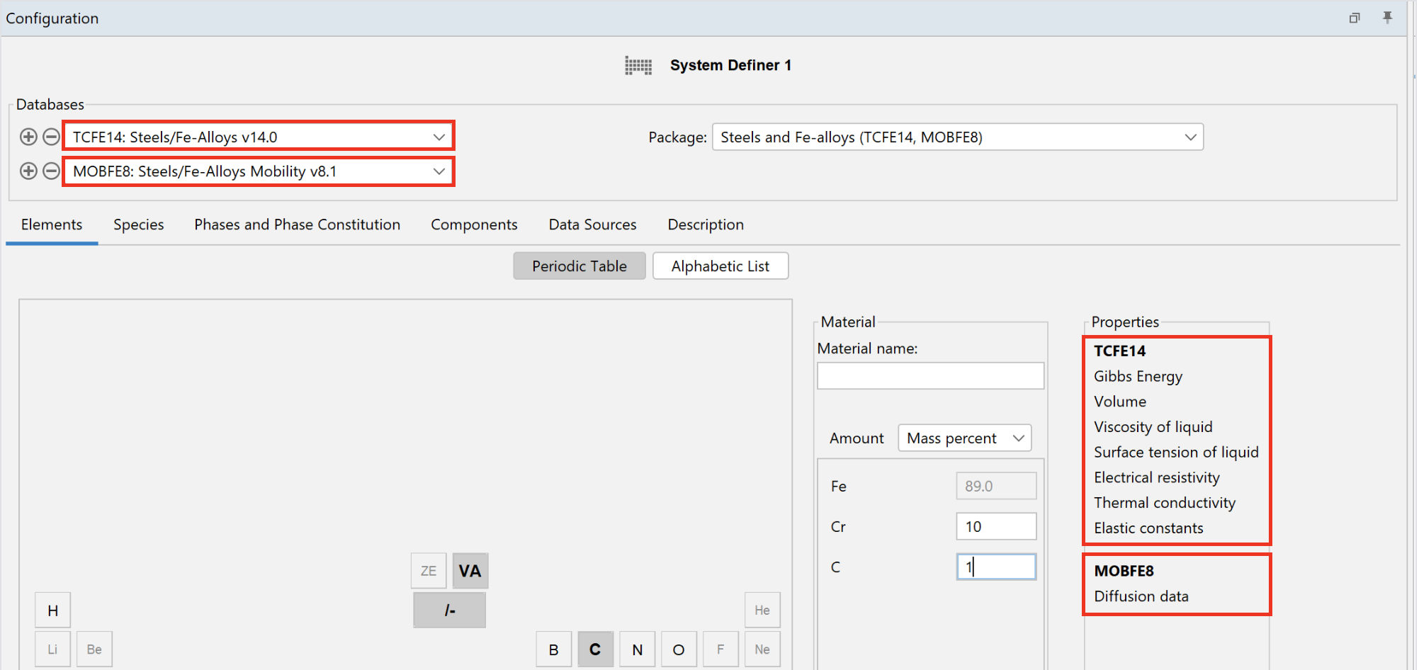
The System Definer in Thermo-Calc showing the new properties lists for the Steel and Fe-alloys databases TCFE14 and MOBFE8.
Reverse Axis Option Fixed in Ternary Diagrams and Simplified in All 2D Diagrams
Several users have requested the ability to reverse the axes in ternary diagrams, which is particularly useful when comparing our plots with those found in scientific journals. This functionality was already available in most other 2D diagrams in the software by manually entering the axis limits in reverse order. This functionality has now been added to ternary plots. Additionally, a Swap button has been added to the plot renderer under Show more for all 2D diagrams to make the process even easier.
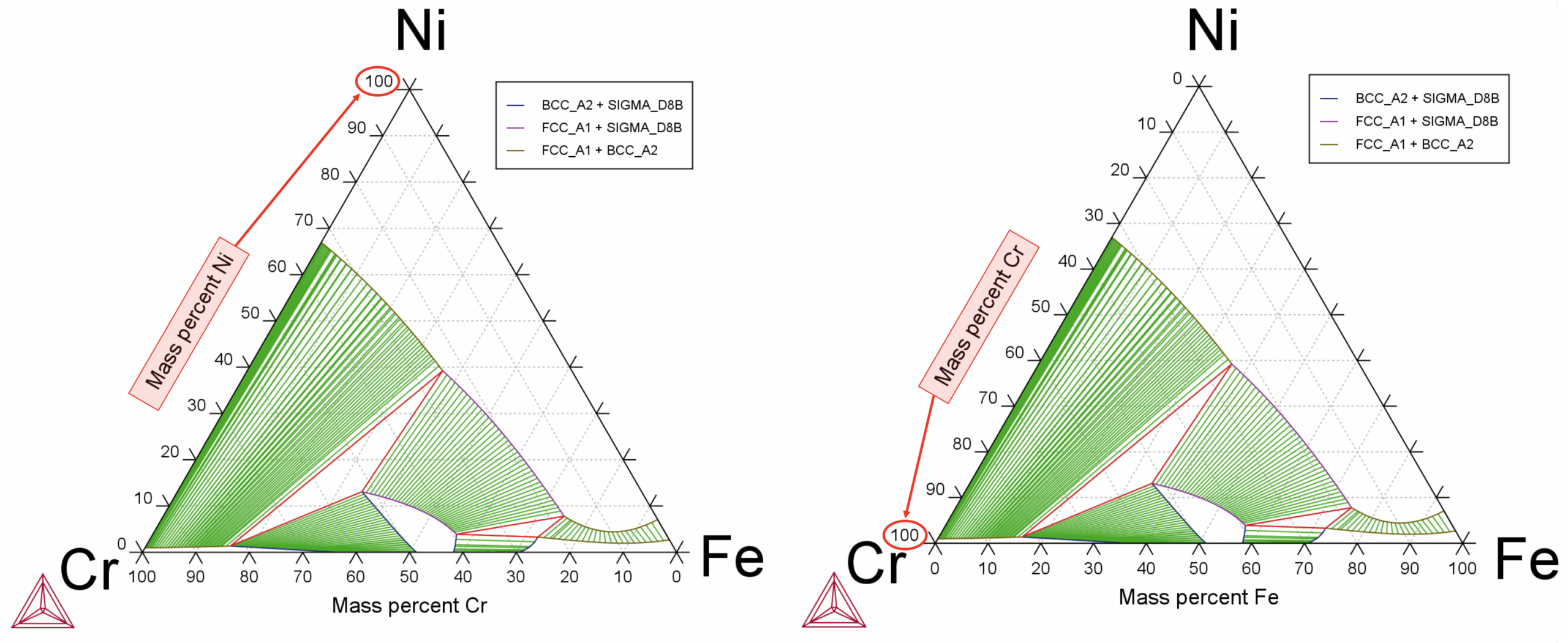
Users can now reverse the axes in ternary diagrams, as shown in the Fe-Cr-Ni diagram, allowing for easy comparison between Thermo-Calc calculations and external sources, such as plots found in publications.
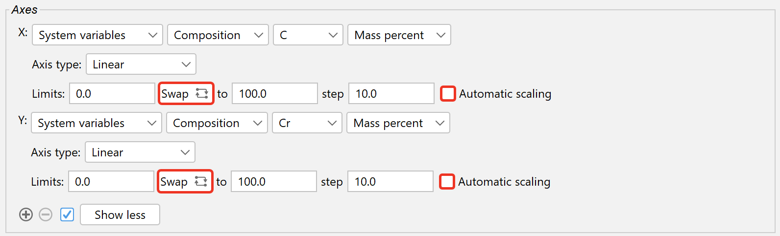
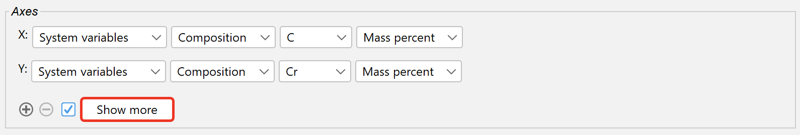
The plot renderer window showing the new Swap button (top), which allows users to reverse the axes in 2D diagrams. Users must select the Show more button (bottom) then uncheck Automatic scaling (top) to enable the Swap button.
Steel Model Library adds Flow Stress Model for Martensitic Steels
The Martensitic Steel Strength Model has been extended to a full flow stress model in this release, able to predict stress at arbitrary strain in the form of the following properties:
The model is also equipped with a mode to predict engineering properties such as:

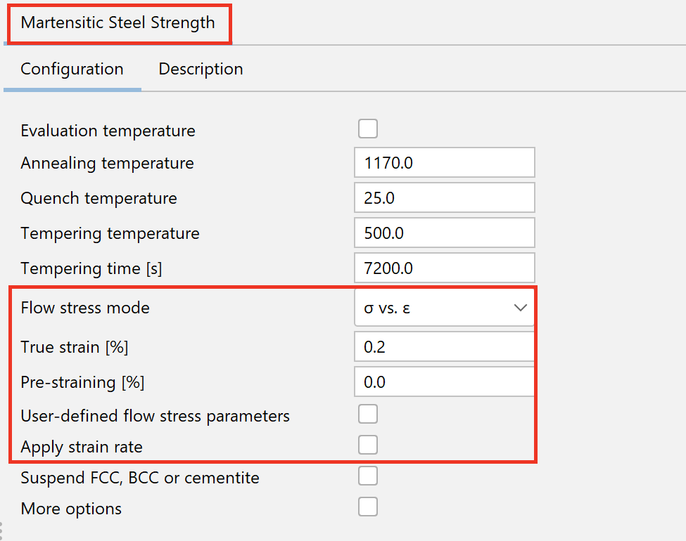
Flow stress curves calculated at 2, 5, and 50 hours for a 15-5PH steel alloy (left) using the new settings in the Martensitic Steel Strength Model, including Flow stress mode, True strain, and Pre-straining (right).
Note: True strain is not available as an input parameter when using the engineering properties mode.
Additional updates and changes have been made to the model to accommodate this valuable extension, which you can read about in the Release Notes.
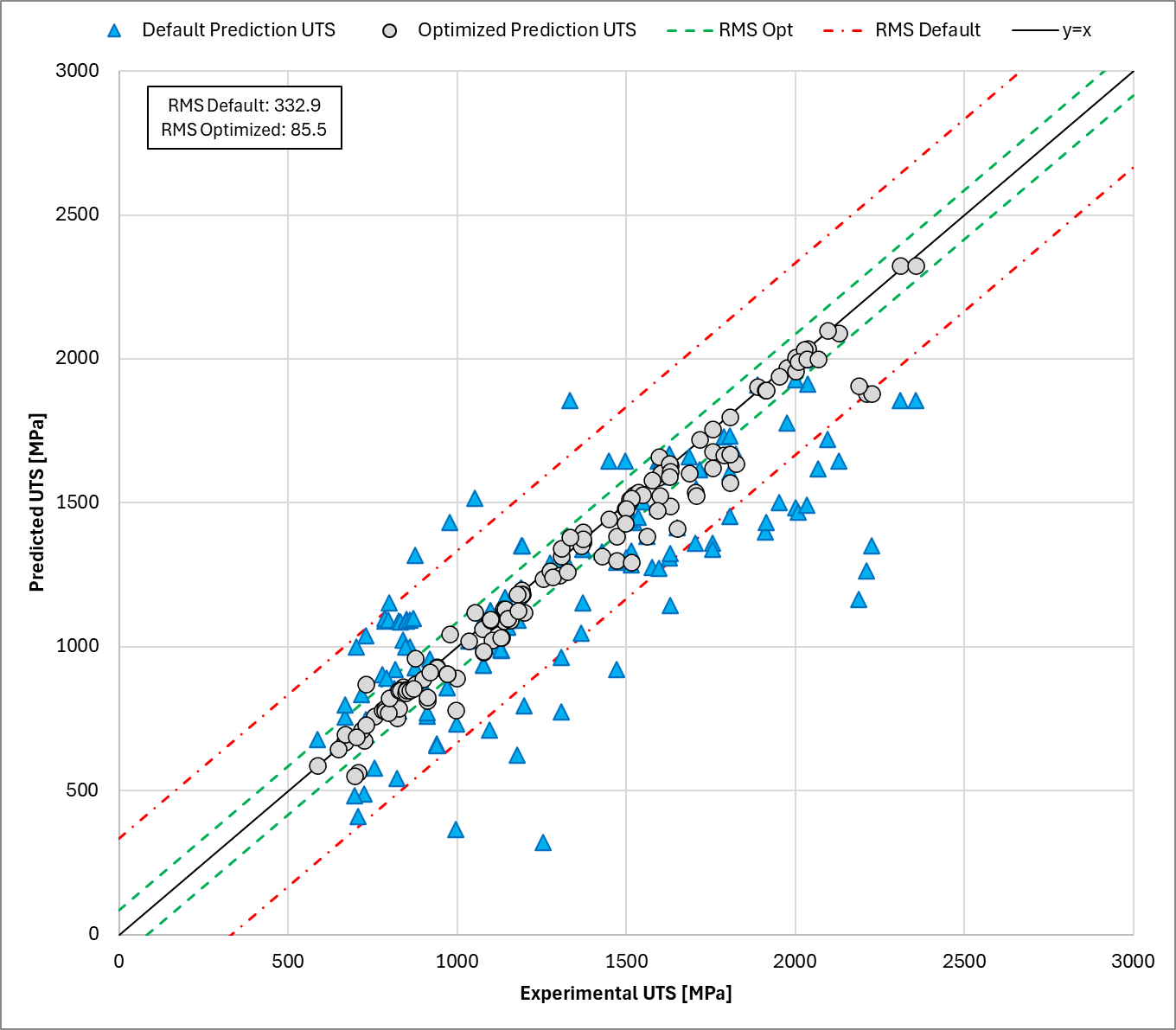
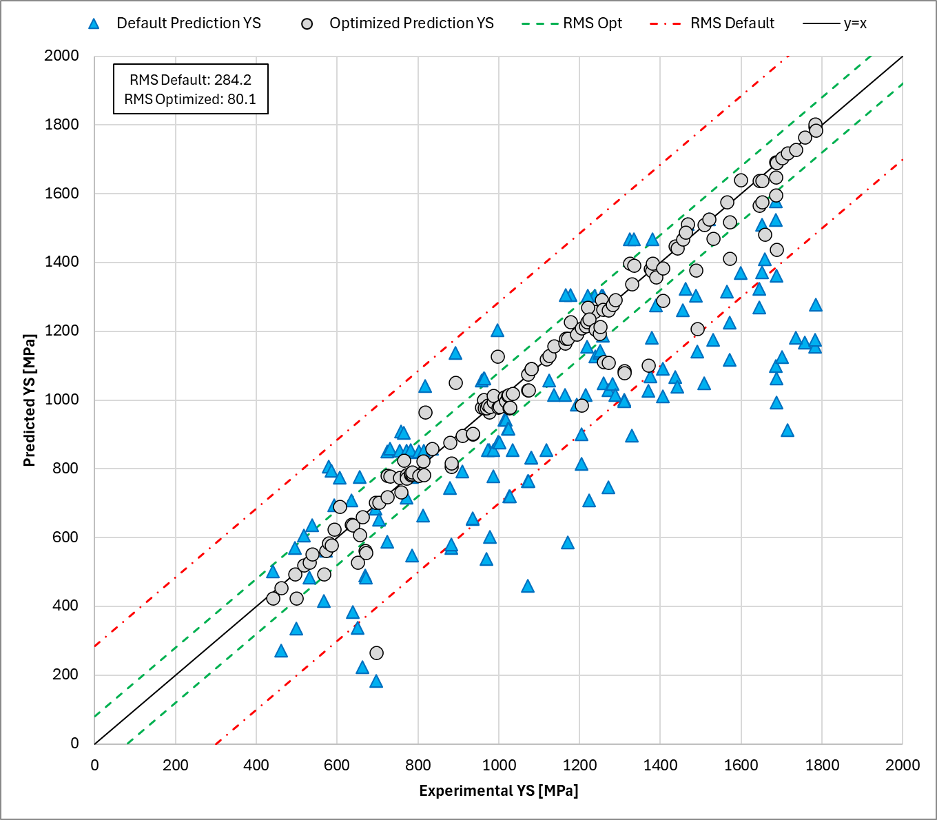
Predicted versus experimental Ultimate Tensile Strength (left) and Yield Strength (right) using default settings versus optimized settings and their respective RMS error. Calculated using the new Flow Stress Model.
Diffusion Module (DICTRA) adds Automatic Grid Placement and Improved Visualization in the GUI
A new Automatic grid option is available in the GUI version of the Diffusion Module (DICTRA), which means the program will automatically distribute the grid points for a calculation. Previously, the only option was for users to set the grid placement manually. This feature was already available in Console Mode and is now also available in Graphical Mode. When you use this feature, you then select whether the size of the grid will be coarse, medium, fine, or custom, which is also a new addition in Console Mode.
Additionally, the program now displays the smallest and largest grid spacing points when hovering over the grid point visualization, as shown in (2) in the image. Some information about the region was already provided, but this additional information was added to prevent users from setting a combination with too many grid points and a high geometric factor that could lead to unusable grid point spacings.
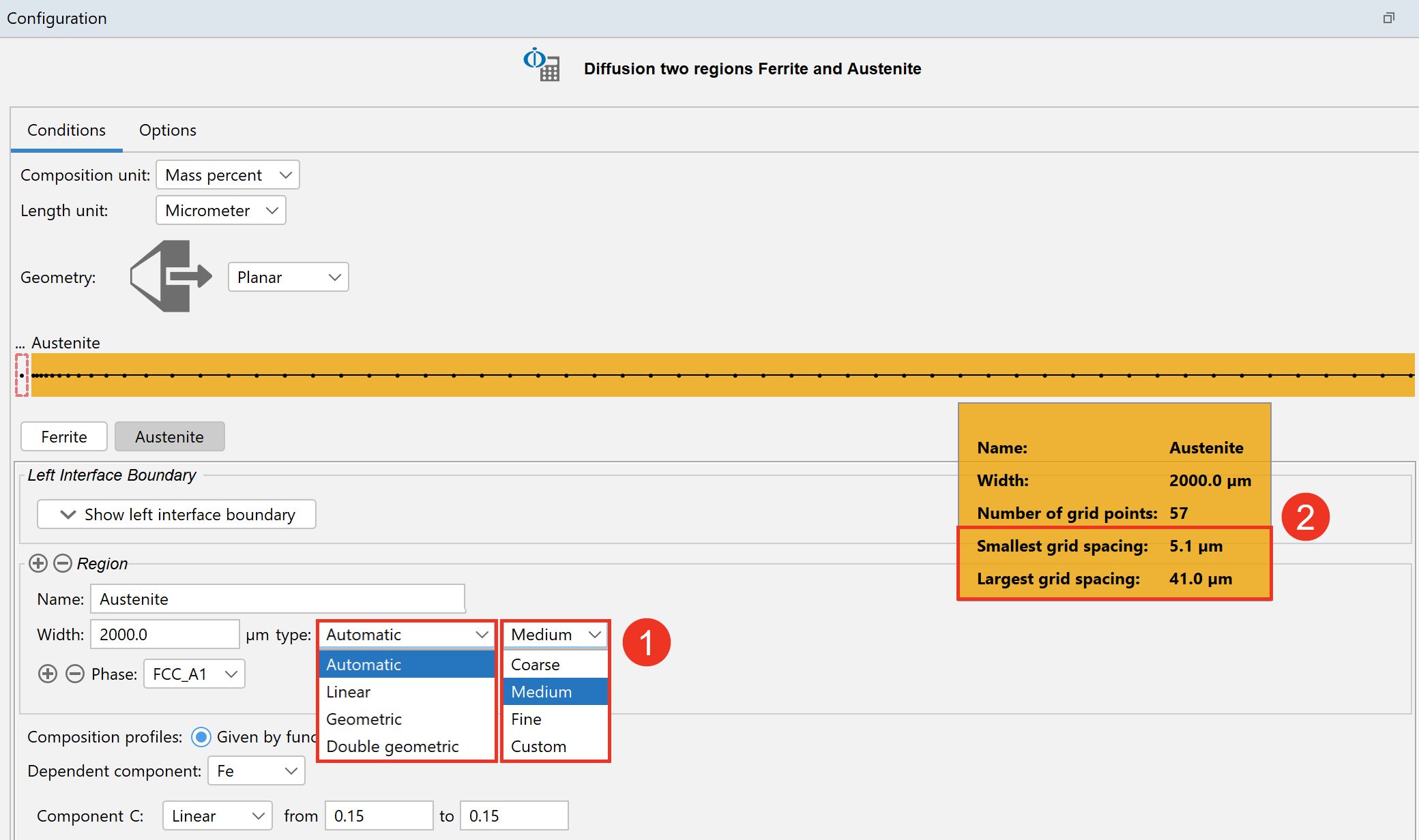
The Diffusion Module (DICTRA) Configuration window, showing the new Automatic grid placement feature (1) and the newly added Smallest and Largest grid spacing points (2).
Precipitation Module (TC-PRISMA) Receives Significant Speed Improvements and Improved Meshing
Speed Improvements
The Precipitation Module (TC-PRISMA) receives a significant improvement in computation speed for non-isothermal simulations. For example, the computation time to simulate a solid solution treatment with a two-step aging of IN718 has been reduced by more than 80% compared to 2025a, as shown in the image.
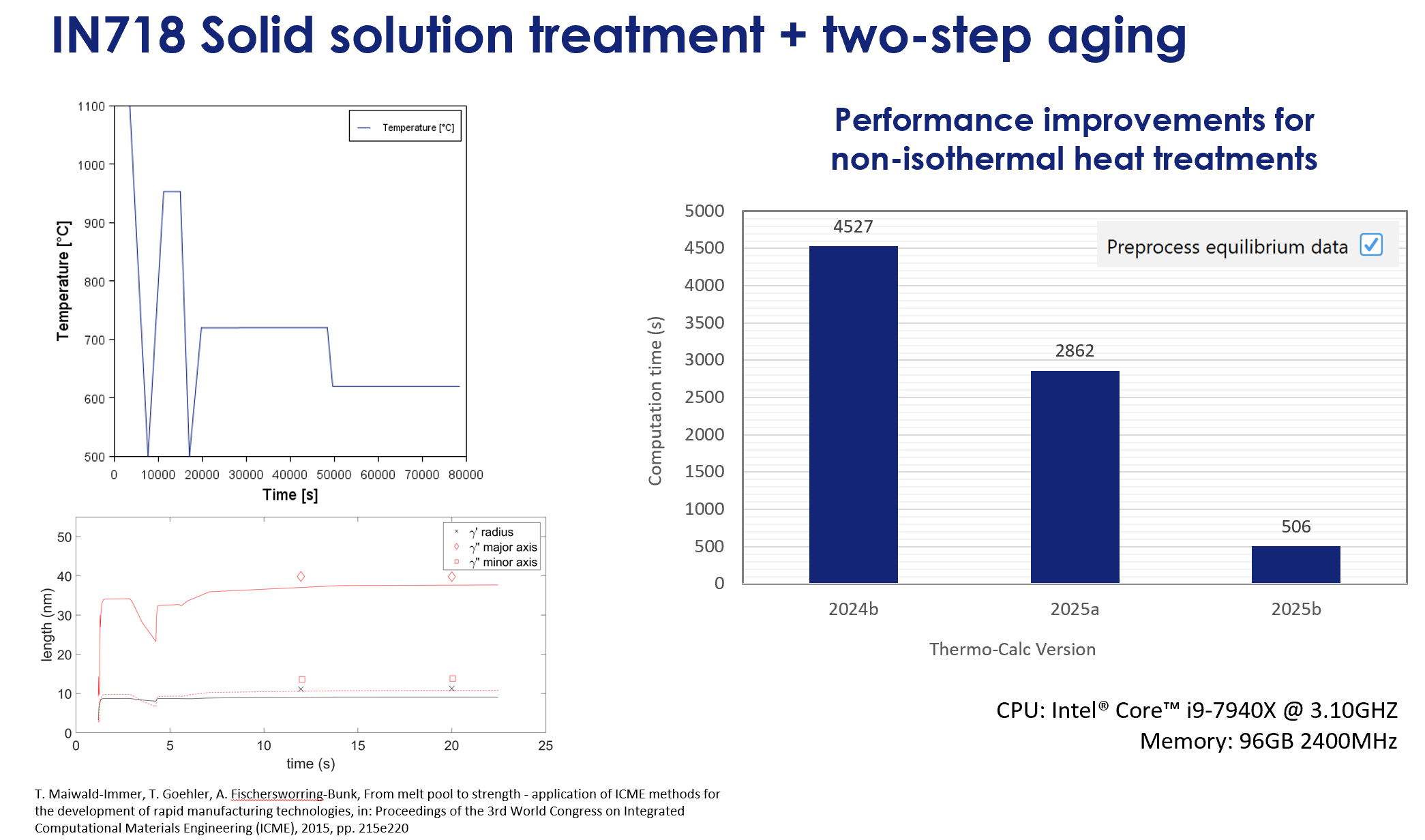
Improvements have been made to the computation time for non-isothermal simulations. For example, simulating the solid solution treatment and two-stage aging of gamma prime, gamma double prime, and delta in IN718 has reduced from 4500s in 2024b to 500s in 2025b.
Improved Meshing
An improvement has been made to the meshing of precipitate size distributions when using PE and PE-automatic growth rate options to make results more accurate. This improvement can be seen in examples P_13 and P_15, which are included in the software.
![Two plots showing a comparison between the measurements of mean cementite radius from [2007Miy] with the simplified (OE), para-eq (PE), and PE Automatic (PE-OE) growth models. Left is from Thermo-Calc 2025a and right is from 2025b, after accuracy improvements were made to the meshing of precipitate size distribution.](https://thermocalc.com/wp-content/uploads/Images/Plots/p-15-2025a-vs-2025b.svg) Two plots showing a comparison between the measurements of mean cementite radius from [2007Miy] with the simplified (OE), para-eq (PE), and PE Automatic (PE-OE) growth models. Left is from Thermo-Calc 2025a and right is from 2025b, after accuracy improvements were made to the meshing of precipitate size distribution.
Two plots showing a comparison between the measurements of mean cementite radius from [2007Miy] with the simplified (OE), para-eq (PE), and PE Automatic (PE-OE) growth models. Left is from Thermo-Calc 2025a and right is from 2025b, after accuracy improvements were made to the meshing of precipitate size distribution.
User Defined Expressions for Interfacial Energies of Precipitate Phases added to TC-Python
It is now possible to create user defined expressions for interfacial energies of precipitate phases in TC-Python for use in the Precipitation Module.
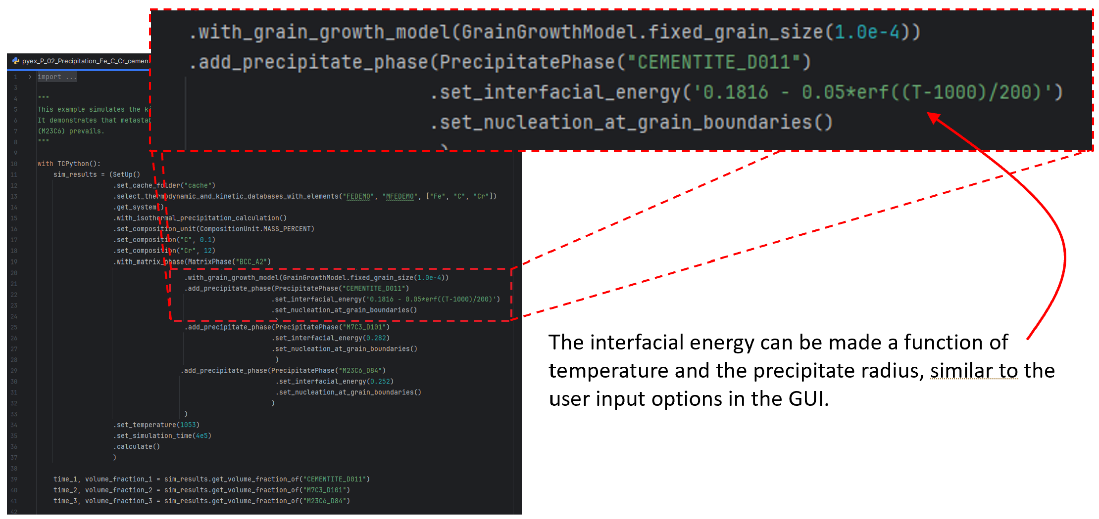
A calculation in TC-Python showing an example of the new user defined expressions for interfacial energies of precipitate phases.
Additive Manufacturing Module
New Beam Shapes Added to Heat Source
Two new beam shapes—Top-hat and Core-ring (Doughnut)—have been added to the heat source options in the Additive Manufacturing Module, offering enhanced control over energy distribution during the printing process.
Gaussian beam distribution in additive manufacturing often leads to high energy intensity peaks and strong thermal gradients, causing manufacturing defects such as keyhole porosity and suboptimal material processing performance. To overcome these challenges, spatial beam shaping is proposed as an alternate method.
The Top-hat beam shape provides a flat, uniform energy distribution within a circular region, while the Core-ring beam shape distributes energy between a central core and an outer ring. The primary benefit of these new beam shapes is a much wider and stabler melt pool. This allows users to increase the productivity of the process so that one can print faster, thus reducing the cost of printing.
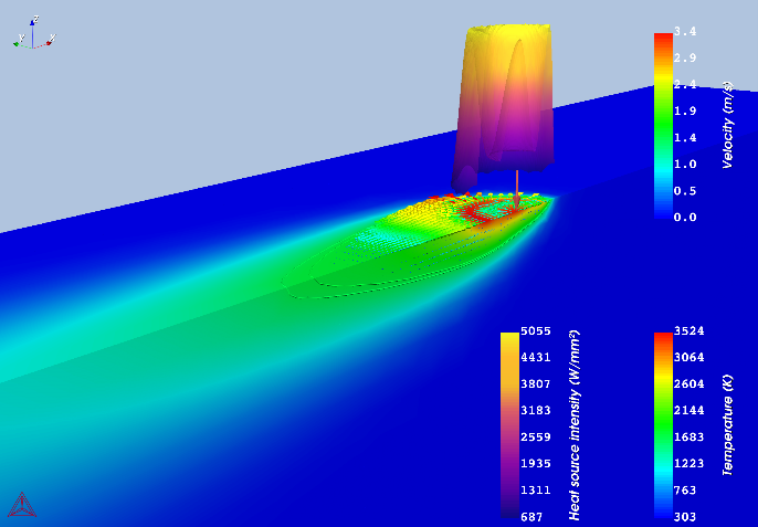
Left: Visualizes the intensity of the Core-ring heat source before the simulation. Index mode 4 is used where 70% of the power is in the ring. Right: Shows the simulated result for 316L at 200 W power, 500 mm/s speed and Custom Core-ring mode with 80% of power in the ring.
Two new examples are available demonstrating the new beam shapes:
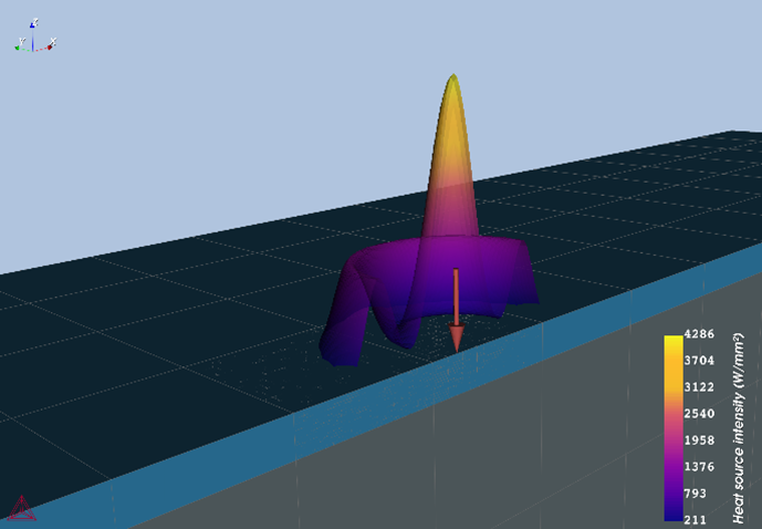
Heat Source Intensity Can be Visualized on 3D Plots
Along with the introduction of the new heat source beam shapes, the heat source is now shown as a heat map of the surface intensity on 3D plots for Gaussian, Core-ring, and Top-hat when the Show Heat Source button is toggled on. An accompanying legend is also included in the plot, as shown in the images above.
Improved Raytracing in Keyhole Model
The raytracing model has been improved in this release. The previous model, based on Jahn, et al (2020), used a stable but simplified approach when accounting for multiple reflections within the keyhole, where rays reflected upwards in the keyhole were ignored. The new approach accounts for full raytracing including upward reflecting rays. The new model changes the shape of the keyhole, which often results in a slightly deeper keyhole and melt pool, as shown in the right image below.
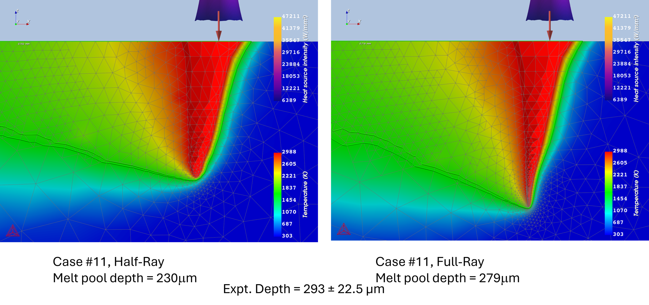
Melt pool depth simulated with half-ray using Thermo-Calc 2025a (left) and full-ray reflect using Thermo-Calc 2025b (right) models compared to experimental depth. Experimental samples printed on an EOS M290 at 336 W power, 750 mm/s speed and 80 µm layer thickness.
Rayleigh Length Improved for Better Consistency with AM Machine Settings
The quantity Rayleigh length has been removed from the Use keyhole model settings for the AM Calculator. A new quantity, Beam quality factor M2, is added in its place. The Rayleigh length is now computed using beam radius, wave length, and M2 when users enter the Beam quality factor M2. This has been done to make the keyhole model consistent with the AM machine settings.
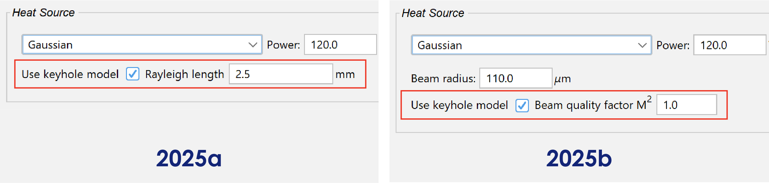
In Thermo-Calc 2025b, Rayleigh length was removed from the Use keyhole model setting in the AM Module and replaced with Beam quality factor M2 in order to improve consistency with AM machine settings and to accommodate for the new heat source beam shapes.